Exploring Music Classification - Composers and Genres
CS 4641 Machine Learning, Team 6, Final Report
Members: Austin Barton, Karpagam Karthikeyan, Keyang Lu, Isabelle Murray, Aditya Radhakrishan
Table of Contents
- Exploring Music Classification - Composers and Genres
- Table of Contents
- References
Introduction
This project addresses the challenges of music audio classification through two distinct tasks on Kaggle datasets, MusicNet and GTZAN. For GTZAN, the objective is genre classification, while for MusicNet, the focus is on identifying composers from the baroque and classical periods. Notably, recent advancements in classification have achieved approximately 92% accuracy [4.], surpassing previous struggles to breach the 80% mark [1.], [2.]. While neural networks dominate current implementations, our study revisits the efficacy of decision trees, particularly gradient-boosted trees, which have demonstrated superior performance in comparison on some cases.
In addition to model exploration, our project delves into data analysis and pre-processing techniques. Both linear and non-linear dimensionality reduction methods are considered, inspired by Pal et al’s., [3] approach. We adopt t-SNE and PCA for dimensionality reduction, leveraging their ability to unveil underlying patterns in the data. We assess and compare the results of these methods visually.
The primary focus of our work lies in comprehensive data pre-processing and visualization. We employ PCA as the primary dimensionality reduction technique, aiming to establish baseline results using minimally processed data with straightforward Feedforward Neural Network architectures. This approach contributes to the understanding of audio (specifically, music audio) datasets and opens questions and important notes for future improvements in music audio classification tasks, emphasizing the potential of decision tree models (and their variants) and the significance of effective dimensionality reduction techniques. Our findings also open up for models specific to sequential data.
Datasets
MusicNet: We took this data from Kaggle. MusicNet is an audio dataset consisting of 330 WAV and MIDI files corresponding to 10 mutually exclusive classes. Each of the 330 WAV and MIDI files (per file type) corresponding to 330 separate classical compositions belong to 10 different composers from the classical and baroque periods. The total size of the dataset is approximately 33 GB and has 992 files in total. 330 of those are WAV, 330 are MIDI, 1 NPZ file of MusicNet features stored in a NumPy array, and a CSV of metadata. For this portion of the project, we essentially ignore the NPZ file and explore our own processing and exploration of the WAV and MIDI data for a more thorough understanding of the data and the task. Further discussion of the data processing is described in detail in the Data Preprocessing section.
Because of how poorly distributed this data is, and not being able to gather new data ourselves, we opted to only do composer classification on a subset of the original data. Any composer with less than 10 pieces in the dataset was completely excluded. This resulted in reducing the number of composers/classes from 10 to 5. The remaining composers are Bach, Beethoven, Brahms, Mozart, and Schubert. This subset is still heavily imbalanced, as Beethoven has over 100 samples of data but Brahms has 10.
GTZAN: GTZAN is a genre recognition dataset of 30 second audio wav files at 41000 HZ sample rate, labeled by their genre. The sample rate of an audio file represent the number of sample, or real numbers, that the file represent one second of audio clip by. This means, for a 30 second wav file, the dimensionality of the dataset is 41000x30. The data set consists of 1000 wav files and 10 genres, with each genre consisting of 100 wav files. The genres include disco, metal, reggae, blues, rock, classical, jazz, hiphop, country, and pop. We took this data from Kaggle.
Overview of Methods and Data Processing
- We utilize Principal Component Analysis on both datasets as our dimensionality reduction technique for visualization as well as pre-processing data.
- We implement t-distributed Stochastic Neighbor Embedding (t-SNE) and compare with PCA.
- We implement classiciation on the MusicNet dataset using decision trees, random forests, and gradient-boosted trees.
- We implement classification on the GTZAN dataset using Feedforward Neural Networks/MLPs on WAV data and Convolution Neural Networks on Mel-Spectrogram PNG images.
- Further discussion of these methods is explained in the Data Preprocessing and Classification sections.
Problem Definition
The problem that we want to solve is the classification of music data into specific categories (composers for MusicNet and genres for GTZAN). Essentially, the existing challenge is to improve previous accuracy benchmarks, especially with methods beyond neural networks, and to explore alternative models like decision trees. Our motivation for this project was to increase classification accuracy, improve the potential of decision trees in this domain, and to better understand and interpret the models that we chose to use. Our project aims to contribute to the field of music classification and expand the range of effective methodologies for similar tasks.
Despite the dominance of neural networks in recent works, there’s motivation to enhance their performance and explore if combining methods can gain better results. The references and readings suggest that decision trees, especially gradient-boosted ones, might perform comparably and offer advantages in terms of training time and interpretability. Based on this, the project aims to effectively reduce the dimensionality of the datasets, enhancing the understanding and visualization of the data using techniques like t-SNE and PCA.
Data Preprocessing
MusicNet:
MIDI Files
For the MIDI files, we aimed to create an algorithm to parse through MIDI files and convert into row vectors to be stored into a data matrix X. We utilize the MIDI parsing software from python-midi to parse through the MIDI files and obtain tensors of float values that corresond to the instrument, the pitch of the note, and the loudness of the note. Each MIDI file generated a (Ix Px A) tensor stored as a 3-D numpy array where I is the number of instruments, P is the total number of pitches, which range from (1-128), and the total number of quarter notes in the piece A. I is held as a constant of 16. For any instrument not played, it simply stores a matrix of zeroes. Additionally, the number of quarter notes in each piece is vastly different. Therefore, we require a way to process this data in a way that is homogenous in its dimensions.
We take the average values of each piece across the 3rd dimension (axis = 2) generating a 2-D array of size 16x128 where each entry is the average float value for that corresponding pitch and instrument across every note in the piece. From here, we flatten the 2-D array to generate a 1-D array of size 16*128 = 2048, where each block of values 128 entries long corresponds to an instrument. This flattening procedure respects the order of the instruments in a consistent manner across all MIDI files and is capable of storing instrument information for all MIDI files within the domain of the 16 instruments. The 16 instruments consist of the most common instruments in classical music including piano, violin, bass, cello, drums, voice, etc. Although the memory is costly, and the non-zero entries in each row vector are quite sparse, we determined that this procedure would be a viable method to maintain information in a manner that is feasible and reasonably efficient for our task.
In summary, we parse through each MIDI file and undergo a basic algorithm to generate row vectors of float values for each composition. We do this for each MIDI file and generate a data matrix X_{MIDI} that is a R^{330x2048} stored as a 2-D array of float values. This data matrix X_{MIDI} is what we will process through supervised models in the future and is the data we further explore with Principal Component Analysis detailed in the next section for MusicNet.
After this processing, filtered out all data belonging to composers with less than 10 pieces in the entire data set. The remaining composers are Bach, Beethoven, Brahms, Mozart, and Schubert and the resulting data matrix is R^{292x2048} This subset is still heavily imbalanced, as Beethoven has over 100 samples of data but Brahms has 10.
WAV Files
For WAV files, we obtain a 1-D array for each song consisting of amplitude float values. Each entry corresponds to a timestep in which the WAV file is sampled which is determined by the sampling rate specified when loading the data. We use the librosa audio analysis package in Python to load WAV files. After data is loaded, take intervals of the WAV data to act as a single data point. The sampling rate is defined as the average number of samples obtained in 1 second. It is used while converting the continuous data to a discrete data. For example, a 30 s song with a sampling rate of 2 would generate a 1-D float array of length 60. If we specify intervals of 3 s, then we would obtain 20 distinct data points each with 3 values (each for amplitude). A possible exploration with this data, because it is sequential, is to use models specifically tailored towards processing sequential data and learning relations between points in a sequence, such as transformers. However, we currently only perform this minimal processing for MusicNet in order to visualize and understand the data, and obtain baseline performances in supervised models to compare to performances with other processed data.
GTZAN:
Extracted Features:
The GTZAN dataset also provides a list of extracted features. There are total of 58 features, which drastically reduces the dimensionality of our input data.
Frequency Space representation using Discrete FFT:
On top of doing supervised learning with the extracted features that the dataset provides, we also directly train on the wav files. To inrease the number of training examples and reduce the dimensionality of the data set, we use 2 second clips instead of the full 30 second clips. To translate the dataset to useful information, we must extract the frequency information. This is because musical notes are made of different frequencies. For example, the fundamental frequency of the middle C is 256 Hz. Translating audio segments into frequencies will allow the model to understand the input much better. To do this, we use a technique called the Fourier Transform. The fourier transform is a way to translate complex value functions into its frequency representations. In our application, we use the finite, discrete version of fourier transform that works on finite vectors rather than functions. In particular, we use a technique called Fast Fourier Transform (FFT) to speed up computation. For every m samples of the 2 second clip, we extract the frequency information from that vector in R^m. We create datasets using m values of 256 and 512. In the end, we end up with a training input of NxTxF, where the first dimension (N) indicates which training sample (2 second clip we are using), the second dimension (T) indicates which of the 256 sample time stamp in the 2 second clip we are in, and the third dimension (F) representing which frequencies (musical notes) are present during that clip.
Dimensionality Reduction - PCA
Principle Components Analysis: Principle Components Analysis (PCA) is a linear dimensionality reduction technique that projects the features of the data along the directions of maximal (and orthogonal to one another) variance. These “new” features are called principle components and are project along what we call principal directions. The principal components can then be ordered by the amount of variance in each principal directions they were projected onto. If we have d dimensions, then we hope to be able to select d’ < d new features that can still effectively separate the data in its corresponding reduced subspace. We choose PCA because of its high amount of interpretability, reasonable computational expensiveness, ubiquitousness, and effectiveness in reducing dimensions while maintaining crucial information and separability of data.
MusicNet: We perform dimensionality reduction using Principal Components Analysis (PCA) on the pre-processed MIDI data. We hope to be able reduce the number of features especially due to the large amount of sparsity in each row vector. Because most of the songs only have 1-2 instruments, which means that for most songs there would be at most 256 non-zero entries, we expect to be able to significanlty reduce the number of features while maintaining separability in our data.
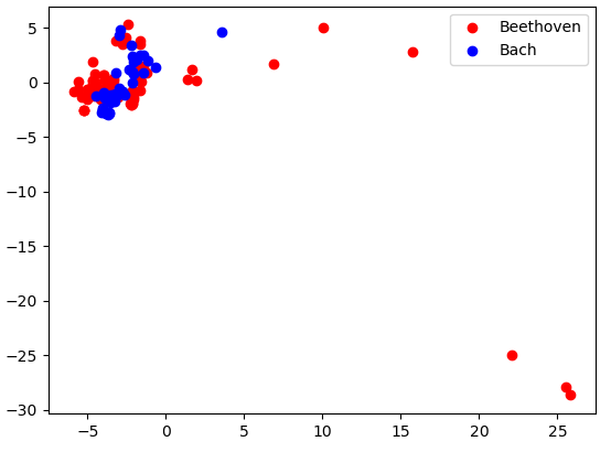
We can see that there is no separation between Beethoven and Bach classes in the first two principal directions.
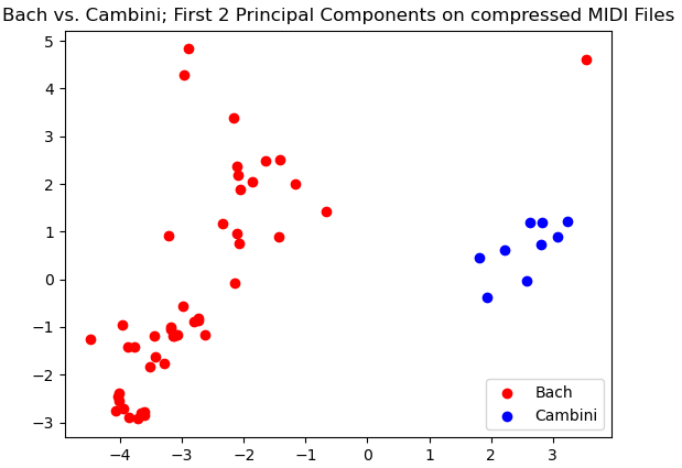
However, very clear separation between Cambini and Bach exists in our data in the first two principal directions.
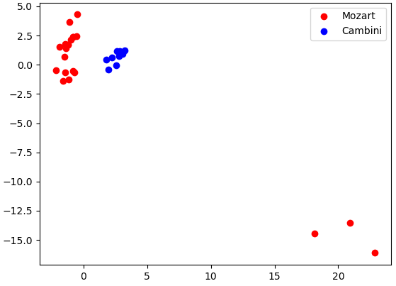
Here we see promising separation between Mozart and Cambini. Although they may not be linearly separable in this case, there is a clear distinction between the clusters of data in our data for their first two principal components.
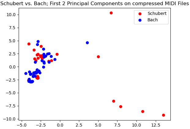
Here again we see a lack of separability for the first two principal components of Bach and Schubert. A strong contrast between Bach vs. Cambini, which did show a high amount of separability. This demonstrates that when performing this classification task on this processed MIDI data, it is likely that the model will struggle to perform well in delineating Bach and Schubert more than it does delineating Bach and Cambini.
GTZAN: After we get our dataset represented by a NxTxF matrix, we perform Principal Component Analysis (PCA) on the dataset. The reason we do this is to reduce the dimensionality of the dataset while mostly maintaining the information we have. This will allow us to train smaller and better models. To do this, we flatten the tensor into a (NT)xF matrix. We then perform PCA to get a (NT)xF’ model. We then reshape it back to a NxTxF’ tensor. We will be testing models utilizing different values of F’.
Dimensionality Reduction - t-SNE
t-distributed Stochastic Neighbor Embedding: t-SNE, or t-Distributed Stochastic Neighbor Embedding, is a dimensionality reduction technique used for visualizing high-dimensional data in a lower-dimensional space, often two or three dimensions. It excels at preserving local relationships between data points, making it effective in revealing clusters and patterns that might be obscured in higher dimensions. The algorithm focuses on maintaining similarities between neighboring points, creating a visualization that accurately reflects the structure of the data. t-SNE is particularly valuable when exploring complex datasets with nonlinear relationships, as it can outperform traditional linear methods like PCA in capturing intricate structures. Note that we only perform t-SNE on the MusicNet dataset.
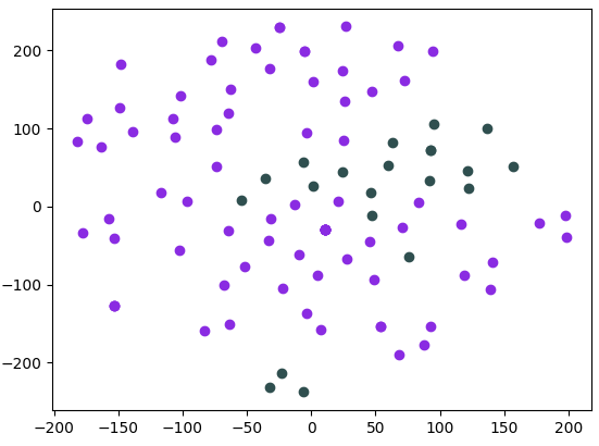
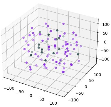
Our t-SNE results were strikingly poor in comparison to the PCA results shown above. In contrast to work by Pal et al., [3], t-SNE performed worse visually than PCA. We demonstrate only one plot for the sake of this report’s brevity, but most class pairs were not linearly separable in 2 or 3 dimensions.
In purple are data points belonging to Beethoven and in green are data points belonging to Mozart.
Here are the data points but in a 3-dimensional space reduced by t-SNE from the original 2048 dimensions.
Classification Methods
MusicNet - Choice of Model and Algorithms:
Chosen Model(s): We decided to use decision trees, random forests, and gradient-boosted trees for our models.
Decision Trees
Methods in this section were inspired from a previous course taken, MATH 4210, and sci-kit learn’s documentation.
Before jumping to more complicated, expensive, and generally less interpretable models, we analyze the results of classification with a single decision tree. Undergoing a proper analysisa dn hyperparametrization of a single decision tree will provide us insight even if the model does not perform well. This will set us up for success and narrow hyperparameter search spaces in the subsequent models.
Decision tree classifiers are models that recursively split data based on features, forming a tree-like structure. Each node represents a decision based on a feature, leading to subsequent nodes. Terminal nodes provide predictions.
| Hyperparameter | Description | Value(s) |
|---|---|---|
criterion | The function to measure the quality of a split | gini |
max_depth | Maximum depth of the individual trees | 10 |
random_state | Seed for random number generation | seed=42 |
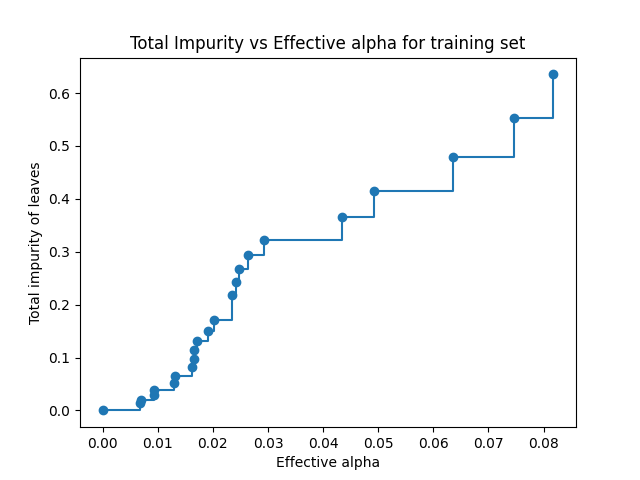
We performed a search over the best value of the cost complexity pruning penalty. This is a penalty coefficient of the complexity of the decision tree, where complexity is measured by the number of leaves in a tree (very similar to ridge and LASSO regression). Below we can see how as we increase the cost complexity hyperparameter (alpha), the total gini impurity of the leaves increases.
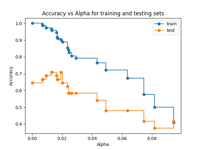
However, this does not mean the model is performing worse as the cost complexity penalty increases. As shown below, there is an optimal cost complexity penality found at around ~0.02 that results in the best test accuracy of the model. This is the cost complexity penalty we use for our decision tree.
Random Forests
Random Forest classifiers are an ensemble learning method combining multiple decision tree classifiers. Each tree is trained on a random subset of data and features. The final prediction is an average or voting of individual tree predictions.
| Hyperparameter | Description | Value(s) |
|---|---|---|
n_estimators | Number of boosting stages to be run | 100 |
max_depth | Maximum depth of the individual trees | 13 |
max_features | Number of features to consider for the best split | 1024 |
random_state | Seed for random number generation | seed=42 |
Since random forests in our case are very computationally feasible, and since our analysis of decision tree performance based on depth provides insight, we opted to search through what max_depth hyperparameter would perform the best. We experimentally found max_depth of 13 to work the best for random forests, in contrast to the best depth for a single decision tree to be 10. Our choice of max_features was based off the fact that many of the data samples are sparse in non-zero entries and only few contain more than 1024 entries (and not by much more) we felt 0.5 to be reasonable and through experimentation found it to be effective.
Gradient-Boosted Trees
Gradient-boosted trees are a type of ensemble learning technique that builds a series of decision trees sequentially, defines an objective/cost function to minimize (very similar to neural network cost functions), and uses the gradient of the cost function to iteratively guide the next sequential tree to improve the overall model. Each tree corrects errors of the previous one and the ensemble model is trained over a defined number of iterations, similar to neural networks. Hence, this model requires lots of hyperparametrization and is in general much more computationally costly compared to decision trees and random forests. Additionally, they are more difficult to interpret.
Model 1 Hyperparameters:
| Hyperparameter | Description | Value(s) |
|---|---|---|
n_estimators | Number of boosting stages to be run | 20 |
learning_rate | Step size shrinkage to prevent overfitting | 0.8 |
max_depth | Maximum depth of the individual trees | 10 |
subsample | Proportion of features to consider for the best split | 0.5 |
objective | The objective function this model is minimizing | multi:softmax |
early_stopping | Stop training early if evaluation doesn’t improve | None |
random_state | Seed for random number generation | seed=42 |
Model 2 Hyperparameters:
| Hyperparameter | Description | Value(s) |
|---|---|---|
n_estimators | Number of boosting stages to be run | 1000 |
learning_rate | Step size shrinkage to prevent overfitting | 0.8 |
max_depth | Maximum depth of the individual trees | 10 |
subsample | Proportion of features to consider for the best split | 0.5 |
objective | The objective function this model is minimizing | multi:softmax |
early_stopping | Stop training early if evaluation doesn’t improve | 100 |
random_state | Seed for random number generation | seed=42 |
eval_metric | Evaluation metrics | auc and merror |
We chose these hyperparameters based off of 1) The results from decision trees and random forests and 2) Our own experimentation searching through the space of possible hyperparameters. These 2 models are essentially the same, but we want to showcase how gradient-boosted trees, although effective, come to limits that adding more iterations will not fix. Our learning rate was tuned through experimentation and searching. The max_depth was experimented with and the results from random forests and decision trees helped guide this selection. We found that including all the features in our model reduced performance and results in the models overfitting extremely fast. Because many of the row vectors are sparse and only few containing more than 1000 entries, we felt 0.5 to be reasonable and through experimentation found it to be effective. We chose the AUC evaluation metric since it does a better job at evaluating classification performance in imbalanced datasets. Lastly, we implement an early stopping of 100 to not waste time and computational resources. The model will stop training and return the best performing model if after 100 iterations the evaluation metrics do not improve.
GTZAN - Choice of Model and Algorithms:
Chosen Model(s): We chose to use deep learning - traditional MLPs that employ human-selected features, and CNNs that classify raw spectrograms.
Multilayer Perceptron
As discussed in our midterm report (from which much of this carries over), we employ a straightfoward feedforward network on the human-selected features. These are not spatially or temporally related, so a model that exploits such structure (CNNs, RNNs, transformers, etc.) in the input is not needed here. It was clear that we had sufficient training samples and a well-balanced dataset, and so a feedforward network seemed effective.
Two variants of the model were built for the two variants of the dataset - 3 and 30 seconds. For both, we employed a 10% validation split to allow monitoring of model performance to detect overfitting. We used early stopping such that if the loss failed to decrease for 3 epochs in a row, the training process would halt.
For both, we employed a softmax activation function (to output a distribution of probabilities - this is a multiclass single-label classification problem) and the categorical cross-entropy loss. Hidden layers used the ReLU activation function, and a variant was not needed as a network so shallow faced little risk from vanishing gradients.
We employed the widely-used Adam optimizer to accelerate convergence.
3-second variant
| Hyperparameter | Description | Value(s) |
|---|---|---|
| Layers | Number of hidden layers in the network | 2 |
n_neurons | Number of neurons in each hidden layer | 512 |
dropout_rate | Dropout rate for regularization | 0.5 |
loss_function | Loss function used | categorical_crossentropy |
optimizer | Optimization algorithm | Adam |
learning_rate | Learning rate for optimizer | 0.001 (1e-3) |
batch_size | Number of samples per batch of computation in training | 32 |
max_epochs | Maximum number of epochs | 500 |
patience | Patience for early stopping (number of epochs) | 3 |
validation_split | Fraction of data to be used as validation set | 0.1 (10%) |
Hyperparameters were chosen largely based on intuition and repeated experimentation.
The iteration over model architectures began with a single hidden layer of 32 neurons. From there, the number of neurons was increased, and as signs of overfitting were noticed, dropout regularization was added in. Not only did this prevent overfitting, but it also improved model performance compared to less parameter-dense networks, likely a consequence of breaking co-adaptations.
However, it is important to note that performance did not climb significantly from a single-hidden-layer network with just 128 neurons and dropout. After this, additional improvements to model capacity provided diminishing returns for the increased needs for computing.
With similar experimentation, it was found (along with optimizer parameters) that the ideal batch size was 32.
30-second variant
| Hyperparameter | Description | Value(s) |
|---|---|---|
| Layers | Number of hidden layers in the network | 2 |
n_neurons | Number of neurons in each hidden layer | 64 |
dropout_rate | Dropout rate for regularization | 0.5 |
loss_function | Loss function used | categorical_crossentropy |
optimizer | Optimization algorithm | Adam |
learning_rate | Learning rate for optimizer | 0.001 (1e-3) |
batch_size | Number of samples per batch of computation in training | 16 |
max_epochs | Maximum number of epochs | 500 |
patience | Patience for early stopping (number of epochs) | 3 |
validation_split | Fraction of data to be used as validation set | 0.1 (10%) |
When dealing with the 30-second variant, the number of training samples drastically reduced, making overfitting an immediate concern. While we ultimately ended up using virtually the same setup (only a smaller batch size, this time 16), we had to make changes to the size and number of layers. The final hyperparameters reflect these changes - a maximum model size for high performance. Anything more complex, and the model tended to suffer from overfitting, and regularization failed to match simpler models.
The 3-second variant essentially represented a better use of the same underlying dataset. It is effectively an augmentation where each 30-second sample is split into 10 parts.
Convolutional Neural Network
Another approach to the GTZAN dataset is to employ raw spectrogram images and use convolutional layers to extract spatial information from them. The CNN is employed here as its filters can learn spatial information in a manner far more efficiently (and effectively) than fully-connected layers.
There were multiple variants to employ here - 256 samples per segment, 512 samples per segment, respective PCA variants, and the raw spectrograms themselves. We categorize these as “processed” for the first four and “raw” for the raw spectrograms.
Similar to the MLP, we employed manual experimentation and trial-and-error via validation performance. This was especially relevant here, where training times were excessive and an architecture search would’ve been highly computationally expensive.
Processed Spectrograms
| Layer Type | Configuration | Description |
|---|---|---|
Conv1D | 32 filters, kernel size 64, activation ‘relu’ | 1D convolutional layer with 32 filters and a kernel size of 64 |
Reshape | Reshape to (-1, 32, 1) | Reshapes the output for subsequent 2D convolutional layer |
Conv2D | 64 filters, (3x3) kernel, activation ‘relu’ | 2D convolutional layer with 64 filters and a (3x3) kernel |
MaxPooling2D | Pool size (2x2) | Max pooling layer with a (2x2) window |
Dropout | Rate 0.2 | Dropout layer with a dropout rate of 0.2 |
Conv2D | 128 filters, (3x3) kernel, activation ‘relu’ | 2D convolutional layer with 128 filters and a (3x3) kernel |
MaxPooling2D | Pool size (2x2) | Max pooling layer with a (2x2) window |
Dropout | Rate 0.2 | Dropout layer with a dropout rate of 0.2 |
Flatten | Flattens the input for the dense layer | |
Dense | 128 neurons, activation ‘relu’ | Dense layer with 128 neurons and ‘relu’ activation |
Dropout | Rate 0.5 | Dropout layer with a dropout rate of 0.5 |
Dense | num_classes neurons, activation ‘softmax’ | Output dense layer with num_classes neurons and ‘softmax’ activation |
The first attempts began with 256 samples per segment variants. While 2D convolutions were initially employed for the entire network, a significant improvement was observed when using 1D horizontal convolutional filters first. The underlying motivation was the idea that each frequency could have its features individually extracted before they were combined in two dimensions. The PCA variant was also experimented with. However, validation set performance had a considerable 20% degradation despite much hyperparameter tuning, and the PCA feature reduced variant was excluded. However, performance was still quite poor, with validation set performance being ~65%.
Attempts with the 512 samples per segment yielded far poorer results, both PCA and otherwise. Many architectures were tried to little avail, and this dataset variant was ultimately abandoned.
Raw Spectrograms
| Layer Type | Configuration | Description |
|---|---|---|
Conv2D | 32 filters, kernel size (3x3), activation ‘relu’ | 2D convolutional layer with 32 filters and a (3x3) kernel |
MaxPooling2D | Pool size (2x2) | Max pooling layer with a (2x2) window |
Conv2D | 64 filters, (3x3) kernel, activation ‘relu’ | 2D convolutional layer with 64 filters and a (3x3) kernel |
MaxPooling2D | Pool size (2x2) | Max pooling layer with a (2x2) window |
Dropout | Rate 0.25 | Dropout layer with a dropout rate of 0.25 |
Conv2D | 128 filters, (3x3) kernel, activation ‘relu’ | 2D convolutional layer with 128 filters and a (3x3) kernel |
MaxPooling2D | Pool size (2x2) | Max pooling layer with a (2x2) window |
Dropout | Rate 0.4 | Dropout layer with a dropout rate of 0.4 |
Flatten | Flattens the input for the dense layer | |
Dense | 128 neurons, activation ‘relu’ | Dense layer with 128 neurons and ‘relu’ activation |
Dropout | Rate 0.5 | Dropout layer with a dropout rate of 0.5 |
Dense | num_classes neurons, activation ‘softmax’ | Output dense layer with num_classes neurons and ‘softmax’ activation |
Here, significant performance improvements were immediately observed, with much cleaner loss graphs and better validation accuracy. Architectures were adjusted and tuned by trial-and-error, tracking overfitting and adding regularization as needed.
The approach of first using 1D filters no longer provided any particular benefit here.
Results and Discussion
MusicNet Results
Decision Trees
We fit our decision tree with the cost complexity hyperparameter described previously. The depth of our resulting tree is 10 (hence, the justification behind this max_depth hyperparameter), providing insight for subsequent models as to how deep a tree should or should not be. The results of this tree are summarized below in a confusion matrix, training and testing accuracy, and F1-score.
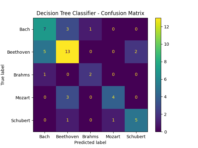
A note on F1-Score and AUC: For this section, we use a weighted average F1-score and weighted average Area Under the receiver operating Curve (AUC). The reason we weight these scores is due to the imbalance in the classes for this dataset. The F1-score metric is the harmonic mean of precision and reall. Thus, it acts as an aggregated metric for both precision and recall. Because it’s defined on a binary case of true/false postive/negatives, each class has its corresponding F1-score. These values are then aggregated by a weighted average into one value, as reported below. The AUC metric is an aggregate measurement of true and false positive rates derived from the ROC plot, which plots the true positive rate (TPR) against the false positive rate (FPR) at each threshold setting. Similarly to the F1-score, this is a binary classification statistics. Therefore, each class has their own AUC score which is aggregated into a single reported AUC. We use both the 1 vs Rest and 1 vs 1 methods. 1 vs Rest divides the data into two classes as the 1 class we are measuring (positive), and the rest (negatives). The 1 vs 1 method only looks at pairwise comparisons between each class as the positives and negatives. Both of the metrics for measuring classification performance are highly regarded and tend to perform better than accuracy alone, especially in imbalanced datasets such as this one [5.], [6.].
Decision Tree Classifier Results:
- Training Accuracy: 1.0
- Test Accuracy: 0.6458333333333334
- Test F1-Score: 0.6475694444444445
- Test 1v1 AUC-Score: 0.7684729549963925
- Test 1vRest AUC-Score: 0.7462224419541492
We can see the model does actually quite well for how little training data there is and how poorly the data is distributed. This landmark shows that our processing algorithm for the MIDI is effective to at least some extent in distinguishing certain composers from others.
Random Forests
Results of random forest classifier described in the classification section.
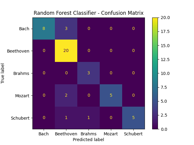
Random Forest Classifier Results:
- Training Accuracy: 1.0
- Test Accuracy: 0.8541666666666666
- Test F1-Score: 0.8519282808470453
- Test 1v1 AUC-Score: 0.9701817279942282
- Test 1vRest AUC-Score: 0.9668985078283857
We can see that random forests drastically improve classification results. Since random forests are highly interpretable and cost efficient, we would opt for this model over other less interpretable and cost ineffecitve models. This idea is showcased in the subsequent section with the introduction of gradient-boosted trees.
Gradient-Boosted Trees
- Boosted-Decision Trees Training Results Model 1 Training Table:
| Iteration | Train AUC | Train Misclassification Error | Eval AUC | Eval Misclassification Error |
|---|---|---|---|---|
| 0 | 0.86054 | 0.36111 | 0.77116 | 0.52083 |
| 1 | 0.93284 | 0.21528 | 0.82366 | 0.47917 |
| 2 | 0.95528 | 0.19444 | 0.84713 | 0.29167 |
| 3 | 0.96822 | 0.17361 | 0.88281 | 0.25000 |
| 4 | 0.97271 | 0.15972 | 0.88940 | 0.31250 |
| 5 | 0.97109 | 0.13889 | 0.90380 | 0.33333 |
| 6 | 0.97126 | 0.15278 | 0.89037 | 0.29167 |
| 7 | 0.97764 | 0.13889 | 0.90454 | 0.27083 |
| 8 | 0.97766 | 0.12500 | 0.92452 | 0.22917 |
| 9 | 0.98132 | 0.12500 | 0.90117 | 0.31250 |
| 10 | 0.98462 | 0.12500 | 0.92574 | 0.25000 |
| 11 | 0.98734 | 0.11806 | 0.92663 | 0.22917 |
| 12 | 0.98723 | 0.08333 | 0.92991 | 0.20833 |
| 13 | 0.98879 | 0.07639 | 0.93026 | 0.22917 |
| 14 | 0.99139 | 0.06944 | 0.93374 | 0.22917 |
| 15 | 0.99309 | 0.07639 | 0.93643 | 0.22917 |
| 16 | 0.99436 | 0.07639 | 0.93824 | 0.20833 |
| 17 | 0.99524 | 0.04861 | 0.93467 | 0.22917 |
| 18 | 0.99714 | 0.05556 | 0.93164 | 0.20833 |
| 19 | 0.99742 | 0.03472 | 0.93645 | 0.20833 |
XGBoost Model 1 Results:
- Training Accuracy: 0.9652777777777778
- Test Accuracy: 0.8541666666666666
- Test F1-Score: 0.7749568668046929
- Test 1v1 AUC-Score: 0.9282258973665223
- Test 1vRest AUC-Score: 0.936447444831591
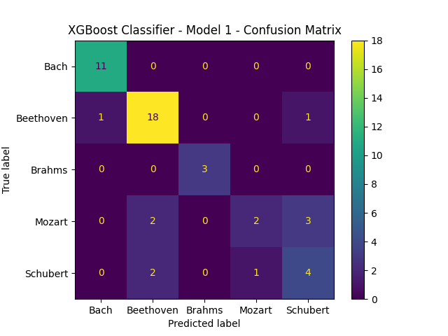
We can see the model does well, but overfits (despite only using half of the features) and does not do better than the random forest implementation we had.
Model 2 Training Table:
| Iteration | Train AUC | Train Misclassification Error | Eval AUC | Eval Misclassification Error |
|---|---|---|---|---|
| 0 | 0.85925 | 0.36111 | 0.77116 | 0.52083 |
| 1 | 0.92848 | 0.22917 | 0.84076 | 0.41667 |
| 2 | 0.94987 | 0.20833 | 0.87133 | 0.27083 |
| 3 | 0.95769 | 0.18056 | 0.89643 | 0.25000 |
| 4 | 0.96958 | 0.15972 | 0.88770 | 0.22917 |
| 5 | 0.96794 | 0.15278 | 0.90044 | 0.31250 |
| 6 | 0.97244 | 0.11806 | 0.88905 | 0.33333 |
| 7 | 0.97616 | 0.11806 | 0.87536 | 0.33333 |
| 8 | 0.98422 | 0.10417 | 0.88341 | 0.33333 |
| 9 | 0.98428 | 0.10417 | 0.88773 | 0.27083 |
| 10 | 0.98491 | 0.09028 | 0.89605 | 0.25000 |
| … | … | … | … | … |
| 160 | 0.99983 | 0.00694 | 0.91817 | 0.22917 |
| 161 | 0.99983 | 0.00694 | 0.91692 | 0.22917 |
| 162 | 0.99983 | 0.00694 | 0.91692 | 0.25000 |
| 163 | 0.99983 | 0.00694 | 0.91742 | 0.18750 |
| 164 | 0.99983 | 0.00694 | 0.91742 | 0.18750 |
| 165 | 0.99983 | 0.00694 | 0.91519 | 0.25000 |
| 166 | 0.99983 | 0.00694 | 0.91418 | 0.25000 |
XGBoost Model 2 Results:
- Training Accuracy: 0.9930555555555556
- Test Accuracy: 0.8541666666666666
- Test F1-Score: 0.7664231763068972
- Test 1v1 AUC-Score: 0.9095452290764792
- Test 1vRest AUC-Score: 0.910000647424428
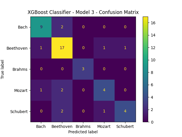
As we can see, training the model more does not result in better performance. Something interesting to note is how, even though they performed the same and the only changed hyperparamter between them is the number of estimators, the confusion matrices are different.
GTZAN Results
Quantitative metrics: 3-second samples
F1 Scores, confusion matrix, etc.
| Genre | Precision | Recall | F1-score | Support |
|---|---|---|---|---|
| Disco | 0.90 | 0.85 | 0.87 | 186 |
| Metal | 0.91 | 0.97 | 0.94 | 199 |
| Reggae | 0.91 | 0.89 | 0.90 | 194 |
| Blues | 0.93 | 0.93 | 0.92 | 190 |
| Rock | 0.90 | 0.83 | 0.87 | 189 |
| Classical | 0.93 | 0.95 | 0.94 | 208 |
| Jazz | 0.89 | 0.91 | 0.90 | 203 |
| Hip Hop | 0.85 | 0.89 | 0.87 | 244 |
| Country | 0.85 | 0.89 | 0.87 | 210 |
| Pop | 0.90 | 0.91 | 0.90 | 183 |
| Accuracy | 0.90 | 1998 | ||
| Macro Avg. | 0.90 | 0.90 | 0.90 | 1998 |
| Weighted Avg. | 0.90 | 0.90 | 0.90 | 1998 |
With a 90% accuray, both weighted and unweighted, this model provides the best results for the entire GTZAN dataset.
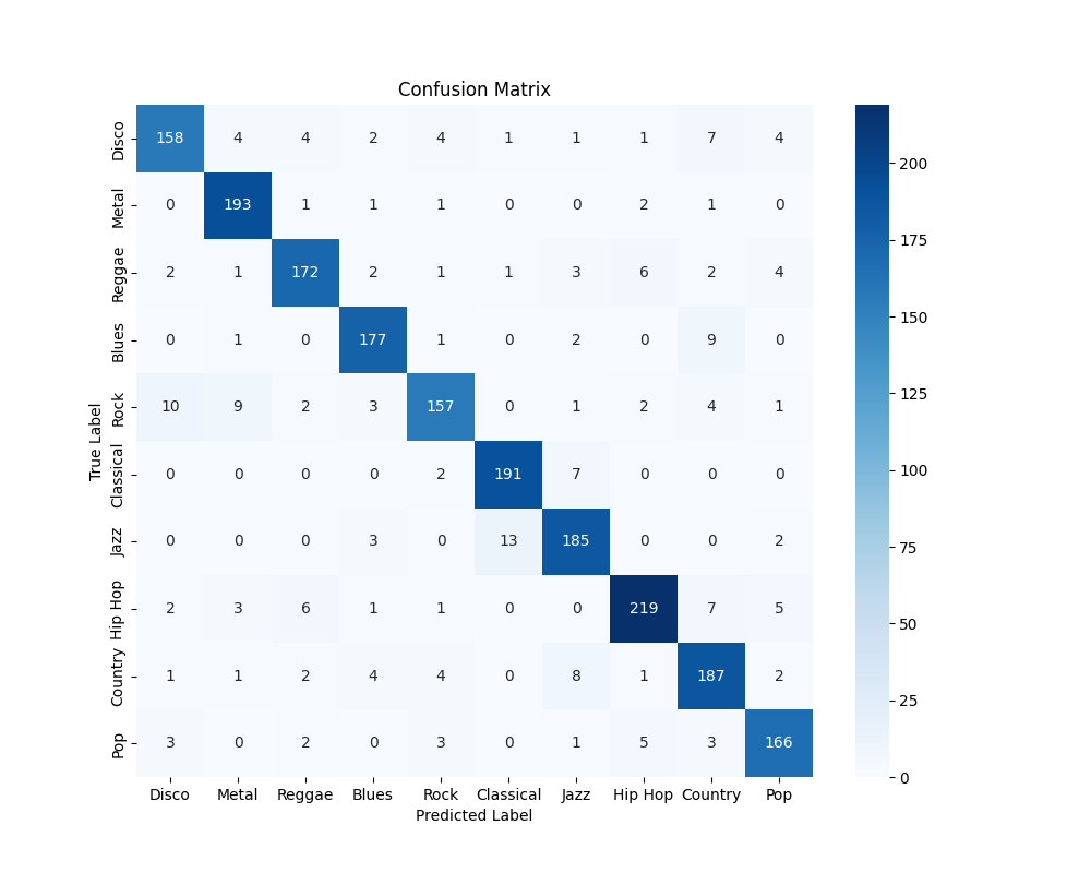
Interestingly, one of the most pronounced type of misclassification is the labelling of rock pieces as either disco or metal, where intuitively, there is a significant amount of similarity.
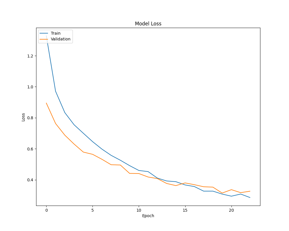
The model has a clean loss graph, and the early stopping prevented the validation loss from continuing to rise.
Quantitative metrics: 30-second samples
F1 Scores, confusion matrix, etc.
| Genre | Precision | Recall | F1-score | Support |
|---|---|---|---|---|
| Disco | 0.67 | 0.48 | 0.56 | 21 |
| Metal | 0.96 | 0.69 | 0.81 | 23 |
| Reggae | 0.79 | 0.75 | 0.77 | 26 |
| Blues | 0.55 | 0.65 | 0.61 | 20 |
| Rock | 0.86 | 0.26 | 0.36 | 19 |
| Classical | 0.56 | 0.90 | 0.68 | 20 |
| Jazz | 0.75 | 0.88 | 0.81 | 17 |
| Hip Hop | 0.65 | 0.79 | 0.71 | 19 |
| Country | 0.76 | 0.61 | 0.68 | 23 |
| Pop | 0.82 | 0.82 | 0.82 | 22 |
| Accuracy | 0.71 | 200 | ||
| Macro Avg. | 0.70 | 0.71 | 0.70 | 200 |
| Weighted Avg. | 0.71 | 0.71 | 0.70 | 200 |
Clearly, as expected and shown by our results with the validation set during model development, performance is considerably worse. This can simply be attributed to fewer training samples, with the model overfitting too quickly before it could adequately learn the underlying function.
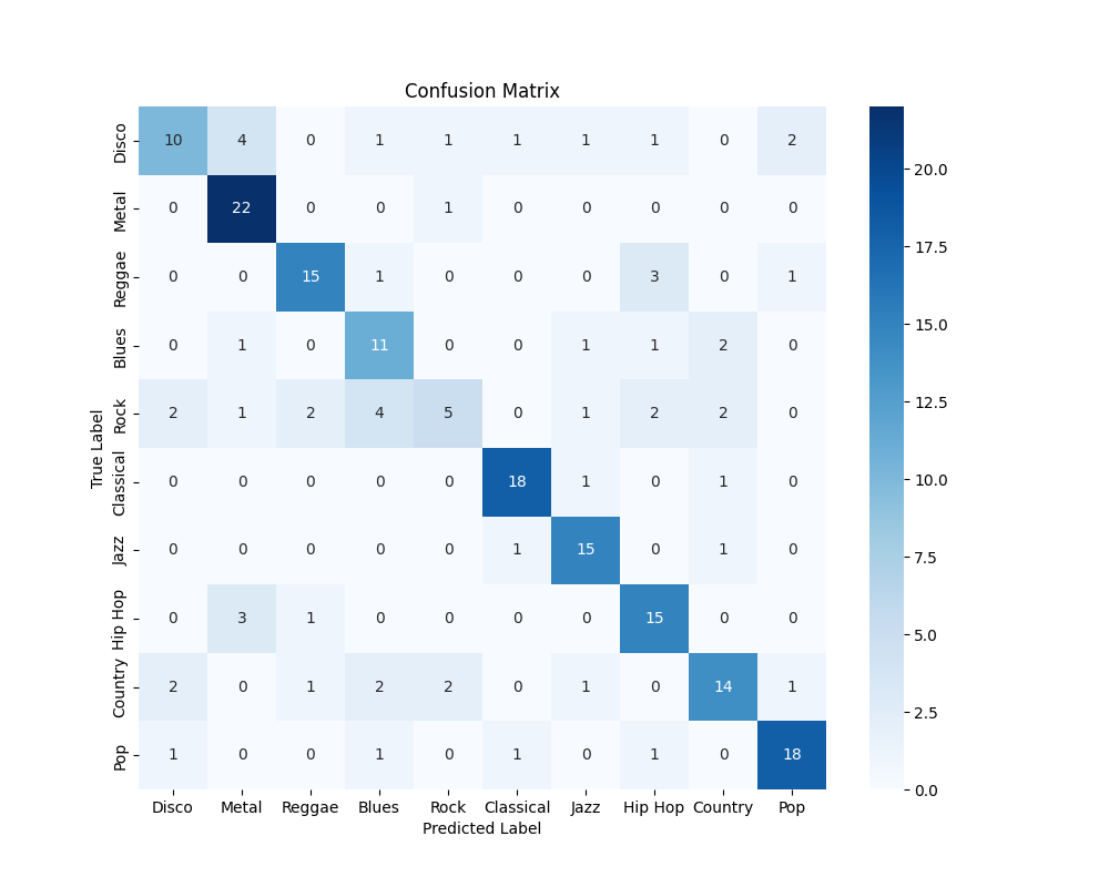
The difficulty of classifying rock is far more pronounced here, although this time, the misclassifications are to classes that are more diverse. However, classes that are highly related to rock (say, blues, from which rock and roll is derived) tend to have a higher misclassification rate than that of, say, classical music. Rock as a genre historically evolved from a number of genres, from jazz to country to blues, and this depth of complexity may be the driving force behind these misclassifications.
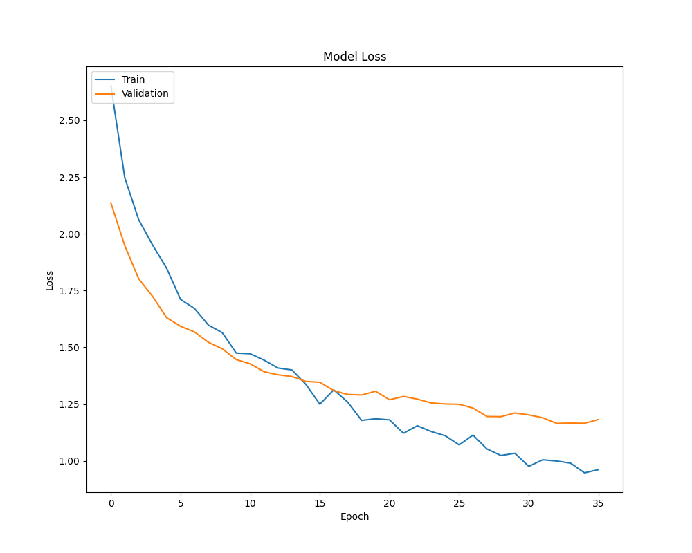
As expected, the loss graph is far worse, with validation loss diverging in a quite pronounced manner from train loss, quickly overfitting.
CNN - Processed Spectrogram (256, non-PCA)
| Genre | Precision | Recall | F1-score | Support |
|---|---|---|---|---|
| Disco | 0.76 | 0.75 | 0.75 | 299 |
| Metal | 0.73 | 0.83 | 0.78 | 293 |
| Reggae | 0.53 | 0.68 | 0.59 | 282 |
| Blues | 0.63 | 0.40 | 0.49 | 300 |
| Rock | 0.46 | 0.30 | 0.36 | 319 |
| Classical | 0.81 | 0.78 | 0.80 | 308 |
| Jazz | 0.52 | 0.62 | 0.57 | 304 |
| Hip Hop | 0.71 | 0.66 | 0.68 | 300 |
| Country | 0.44 | 0.62 | 0.52 | 305 |
| Pop | 0.80 | 0.67 | 0.73 | 287 |
| Accuracy | 0.63 | 2997 | ||
| Macro Avg. | 0.64 | 0.63 | 0.63 | 2997 |
| Weighted Avg. | 0.64 | 0.63 | 0.63 | 2997 |
The CNNs on the processed spectrogram generally perform quite poorly. Extracting features from the raw spectrogram is a far more difficult function to learn than classifying human-selected features, which is effectively much more refined information that humans use when making and playing music. However, the model is certainly far better than a simple randomized classification, and it has certainly learned something.
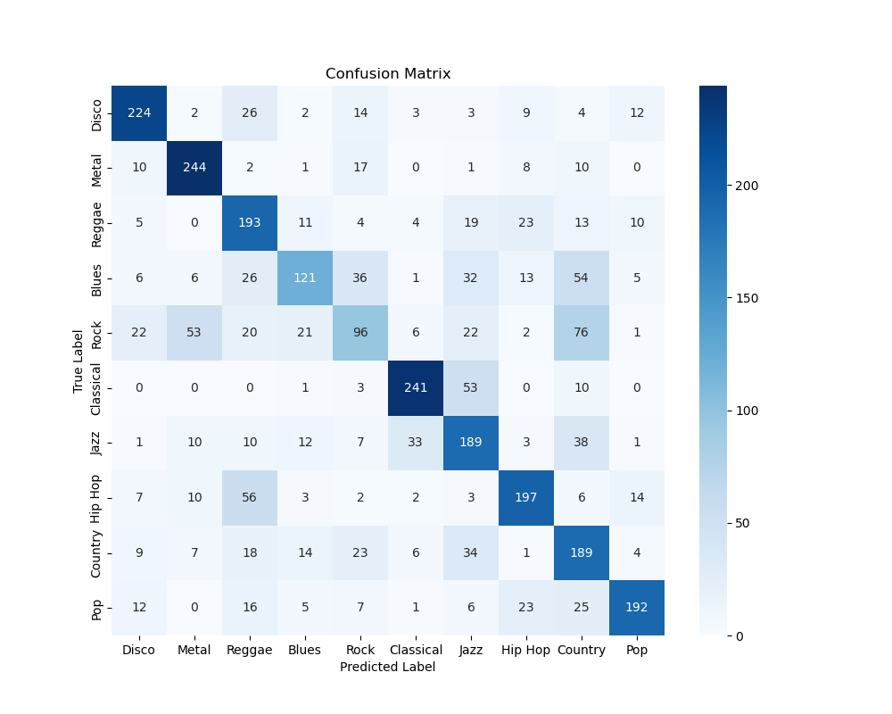
Just as before, rock seems to be misclassified a lot, with blues following not too far behind. Once again, the fact that rock is, in part, derived from blues means that the two are highly similar, and these misclassifications may be explained in this way.
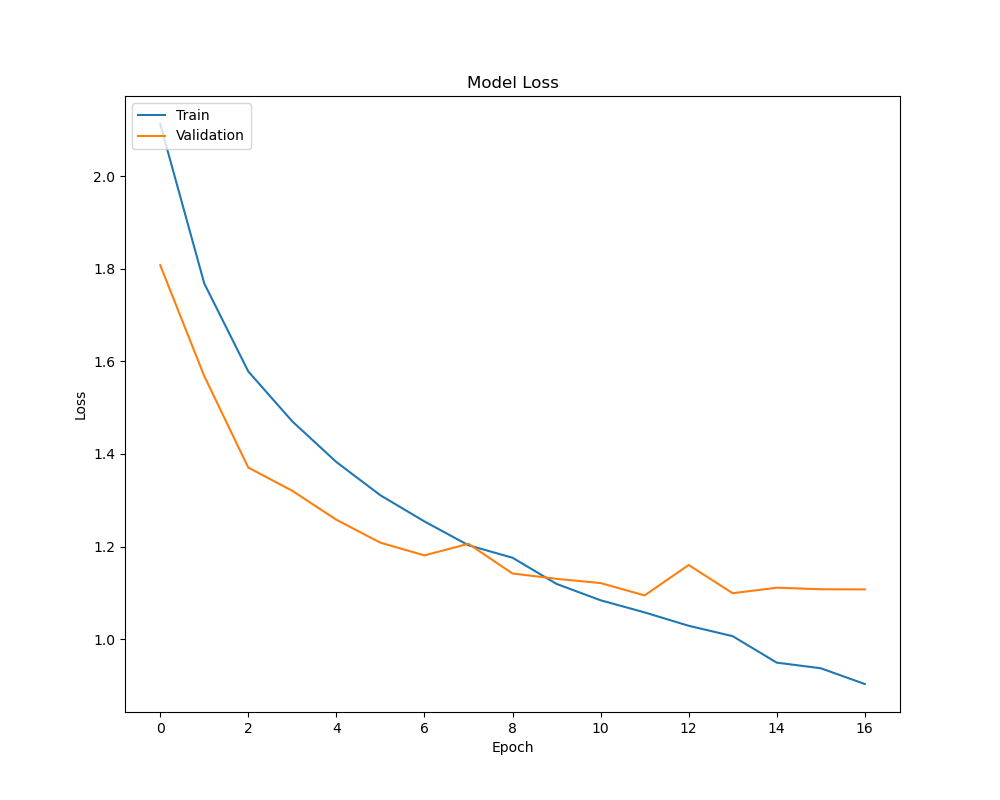
The loss graph considerably diverges at ~8-9 epochs, showing the start of overfitting.
CNN - Raw Spectrogram (2s)
| Genre | Precision | Recall | F1-score | Support |
|---|---|---|---|---|
| Disco | 0.76 | 0.68 | 0.72 | 326 |
| Metal | 0.82 | 0.95 | 0.88 | 300 |
| Reggae | 0.76 | 0.70 | 0.73 | 299 |
| Blues | 0.76 | 0.67 | 0.71 | 316 |
| Rock | 0.64 | 0.56 | 0.60 | 281 |
| Classical | 0.80 | 0.98 | 0.88 | 294 |
| Jazz | 0.85 | 0.75 | 0.80 | 291 |
| Hip Hop | 0.74 | 0.82 | 0.78 | 299 |
| Country | 0.67 | 0.71 | 0.69 | 284 |
| Pop | 0.74 | 0.75 | 0.74 | 307 |
| Accuracy | 0.76 | 2997 | ||
| Macro Avg. | 0.75 | 0.76 | 0.75 | 2997 |
| Weighted Avg. | 0.76 | 0.76 | 0.75 | 2997 |
The raw spectrogram model performs considerably better than the processed ones. This is likely due to the processed spectrograms losing valuable information for classification. However, the inherent greater complexity of this function results in a performance that is still inferior to the best MLP.
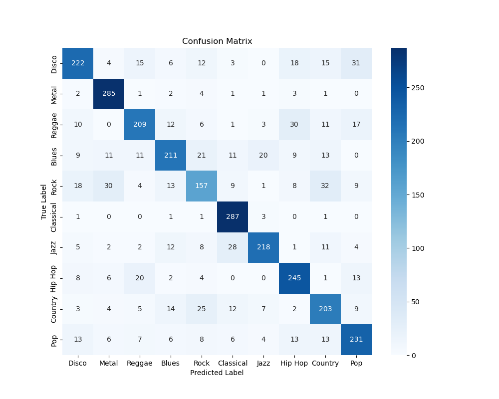
Once again, patterns in rock music being misclassified are observable, a universal trend. The distinct nature of classical music as an archaic genre may help set it apart, resulting in a high model accuracy.
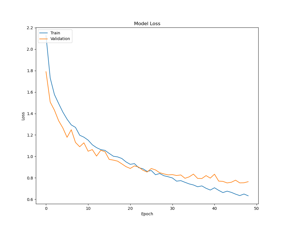
The model has a much better loss graph here, likely due to it being able to learn the function better due to the presence of more information before signs of overfitting creep in.
Discussion
MusicNet: This project focuses on incorporating neural networks to decision trees, random forests, and gradient-boosted trees through a nuanced approach that considers both performance and practicality. The emphasis on the latter models, particularly gradient-boosted trees, indicates a goal of competitive performance while using advantages in training time and interpretability, where this model selection aligns with our broader goal of improving existing accuracy benchmarks, especially through methods beyond neural networks, that ultimately reflects a commitment to contributing to the field of music classification and broadening the range of effective methodologies. The results section provides a clear presentation of the models’ performances, showcasing training accuracy, test accuracy, F1-score, and AUC. The decision tree’s respectable performance despite limited training data and the dataset’s distribution sets a benchmark. The subsequent improvements seen with random forests and gradient-boosted trees highlight the project’s evolution. The comparative analysis between models, especially the observation that increasing the number of estimators in gradient-boosted trees does not necessarily improve performance, offers valuable insights.
We were able to handle the complexities of classical music data through the processing algorithm for MIDI files, transforming them into row vectors and further into a 2-D array for supervised models. While the averaging of values across the third dimension and flattening of the resulting 2-D array present a reasonable solution to the challenge of varying quarter notes in each piece, we can improve this and optimize this algorithm. The discussion of hyperparameters for decision trees, random forests, and gradient-boosted trees adds depth to the project, and the emphasis on fine-tuning these parameters based on model performance sets the stage for a systematic refinement of the models. Overall, the project’s exploration, model choices, and attention to practical considerations definitely contribute to the realm of music classification as a whole.
GTZAN: From the analysis of different models, it’s quite clear that human-extracted features perform better than spectrograms, at least when models are relatively shallow. As discussed before, this is likely owed to the fact that human-extracted features represent handpicked selections that are more representative of how we interpret patterns in music, and differences in these patterns is what we recognize as different genres. A CNN has to implicitly learn this from a spectrogram, which significantly increases complexity.
However, it may well be that spectrograms still provide valuable insights, as they certainly contain more raw information (i.e., the entire piece, just without phase information). As we’ll discuss in “Next Steps”, this fact may be exploited to improve model performance in the future.
Perhaps one of the most interesting insights we find is in how the model does its missclassifications, a finding that is more pronounced in the poorly-performing models. Namely, it is the interesting consequence of rock being a genre that has both a number of predecessor genres (blues, bluegrass, country, boogie-woogie, gospel, and country music) as well as successor genres (pop, metal, etc.). This results in a number of misclassifications for rock, being the “central genre” between these predecessors and successors. Additionally, genres that are not part of this interrelated family end up having performance that is quite high, especially evident with classical music. This potentially shows that the models (however medicore some of their individual performances may be) are learning fundamental features that define western music as an art form.
Overall:
With our project, we implemented several different architectures, with each model crafted towards a specific representation of music - midi, spectrograms, and extracted features. These models were able to extract information from each representation and perform supervised classification on its genre.
Midi, as a logical and intuitive way to organize music, make features such as intervals, chords, and progressions much easier to parse. This prompted us to use techniques that can utilize these structures to its fullest - tree based methods. Raw spectrogram files is a way to represent audio files directly that can be learned by a spectrogram. Our work shows that deep convolutions neural network is able to learn complex features and understand genre. However, due to the large dimensionality of audio files, learning features from spectrogram files requires complex models and large datasets. We were able to get better results by using 1D convolutions to account for music’s unique representation in the frequency domain. We discovered that human selected features by industry experts performed the best. This reflects the paradigm that domain knowledge can boost machine learning methods by significantly reducing the size and simplicity of models, and can perform complex methods trained on raw data.
Our results explores the capabilities of machine learning methods when applied on supervised learning tasks to different representations of music.
Next Steps
MusicNet:
- Fine-tuning Hyperparameters: The decision tree provides a baseline, and the hyperparameter search space can be refined based on its results, and we could do more experimentation with random forests and gradient-boosted trees hyperparameters could potentially improve performance.
- Feature Importance Analysis: For decision trees and random forests, analyzing feature importance can provide insights into which aspects of the data contribute the most to classification, where understanding which musical features are crucial for distinguishing composers can enhance model interpretability.
- Addressing Class Imbalance: The imbalanced distribution of samples among composers, especially evident in the reduced subset, may impact model performance, where techniques like oversampling, undersampling, or using different class weights during training could be further explored, noteably the composers whom have much less data to work with compared to the other composers in the dataset.
GTZAN:
- Improving Performance with Spectrogram Data: Exploring performance improvement with spectrogram data is a promising avenue. Human-extracted features may not benefit significantly from more complex models, as our work shows high performance but diminishing returns. Spectrograms, containing more information, paired with sophisticated models and better preprocessing techniques, could enhance performance further.
- Combining Convolutional Feature Extractor with Human-Extracted Features: A hybrid approach could involve building a model that combines a convolutional feature extractor with human-extracted features. The concatenated features would then be classified by a feedforward network (MLP). This method aims to merge the simplicity of human-derived features with the detailed insights from spectrograms, potentially creating a superior model.
Contribution Table
| Contributor Name | Contribution Type |
|---|---|
| Austin Barton | MusicNet Data Pre-Processing, MusicNet PCA, t-SNE, MusicNet CNN experimentation, Decision Trees, Random Forests, Gradient-boosted trees, Hyperparametrization, Figure generation and analysis, MIDI Parsing, Data Visualization, EDA, GitHub Pages |
| Aditya Radhakrishnan | Model Design & Implementation, Development/Iteration, Validation, Testing, Results Generation & Visualization, and Early Dataset Balancing Exploration |
| Isabelle Murray | GanttChart, Model Implementation/development, Testing, Results Generation & Visualization |
| Karpagam Karthikeyan | MusicNet Data Pre-Processing, Github Pages, Data Visualization, MIDI Parsing, Figure Generation, CNN Model, Video Presentation, GanttChart |
| Niki (Keyang) Lu | GTZAN Data Preprocessing & Visualization |
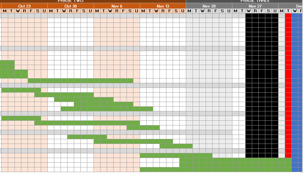
Gantt Chart
Link to Gantt Chart: Gantt Chart

References
[1.] Pun, A., &; Nazirkhanova, K. (2021). Music Genre Classification with Mel Spectrograms and CNN
[2.] Jain, S., Smit, A., &; Yngesjo, T. (2019). Analysis and Classification of Symbolic Western Classical Music by Composer.
[3.] Pál, T., & Várkonyi, D.T. (2020). Comparison of Dimensionality Reduction Techniques on Audio Signals. Conference on Theory and Practice of Information Technologies.
[4.] (https://www.kaggle.com/code/imsparsh/gtzan-genre-classification-deep-learning-val-92-4) Gupta, S. (2021). GTZAN-Genre Classification-Deep Learning-Val-92.4%.
[5.] Ferrer, L. (n.d.). Analysis and comparison of classification metrics - arxiv.org. Arxiv. https://arxiv.org/pdf/2209.05355.pdf
[6.] Brownlee, J. (2021, April 30). Tour of evaluation metrics for imbalanced classification. MachineLearningMastery.com. https://machinelearningmastery.com/tour-of-evaluation-metrics-for-imbalanced-classification/